Developer documentation
OptiFloat.jl implements the Herbie approach to floating-point expression optimization. The steps below outline what the @optifloat macro does. Each step will be discussed in detail throughout this document.
Given an initial Julia expression
expr, compute thelocal_biterrorof every subexpression and identify the subexpressionsub_exprwith the highest error for further analysis.Recursively rewrite
sub_exprbased on aREWRITE_THEORYand simplify it usingSIMPLIFY_THEORY, generating a number of newCandidates.Keep track of all alternatives to
expr(and their associated errors) in a list. Select the next unused expression from that list and start again from step 1. The process concludes after a predefined number of steps or when all alternatives have been tested.Finally, infer good regimes: There may not be a single expression that performs well for all inputs. OptiFloat.jl (like Herbie) infers optimal intervals for the different alternative expressions and produces a compound expression.
Load packages
using DynamicExpressions: parse_expression
using OptiFloat
using Random

# FIXME: sometimes getting NaI in logsample
Random.seed!(1);Random.TaskLocalRNG()Local biterror
OptiFloat.jl computes the biterror of an expression by comparing the exact result of an expression with the 'normal'/'approximate' result (further called floating point evaluation).
Exact evaluation of an expression is done by evaluating it with Interval{BigFloat}s (from IntervalArithmetic.jl) where the precision of the BigFloat is increased until a thin result interval is obtained.
The local_biterror is computed by exactly evaluating the input arguments to a given node op in an expression tree, and computing the biterror between the floating point and exact evaluations of op. In order to evaluate all the operations in an expression tree, we would normally have to walk the tree and eval each node which would be prohibitively slow. To avoid frequent calls to eval for subexpression evaluation we use DynamicExpressions.jl as demonstrated below.
using DynamicExpressions

orig_expr = :((b * (-1) - sqrt(b^2 - 4c)) / (2c))
dexpr = parse_expression(orig_expr;
    binary_operators=[-, ^, /, *, +],
    unary_operators=[-, sqrt, exp, abs, cbrt, log],
    node_type=Node{Float16},
    variable_names=["b", "c"],
)

# OptiFloat defines a convenience overload for the above:
dexpr, features = parse_expression(Float16, orig_expr)

# dynamic expressions are callable with batches of inputs:
points = Float16[
    -2 -50;
     1 1;
]
dexpr(points)
2-element Vector{Float16}:
1.0
0.01563DyanmicExpressions makes it easy to dynamically evaluate subexpressions without loosing performance. We can compute the errors for all sub-expressions:
local_errs = OptiFloat.local_biterrors(dexpr, points)Dict{DynamicExpressions.NodeModule.Node{Float16}, Float16} with 13 entries:
x2 => 0.0
2.0 => 0.0
sqrt((x1 ^ 2.0) - (4.0 * x2)) => 0.0
4.0 => 0.0
x1 ^ 2.0 => 0.0
(x1 * -1.0) - sqrt((x1 ^ 2.0) - (4.0 * x2)) => 4.082
(x1 ^ 2.0) - (4.0 * x2) => 0.0
-1.0 => 0.0
2.0 * x2 => 0.0
x1 * -1.0 => 0.0
((x1 * -1.0) - sqrt((x1 ^ 2.0) - (4.0 * x2))) / (2.0 * x2) => 0.0
4.0 * x2 => 0.0
x1 => 0.0Sample test inputs
Samples/points are batches of vectors with length arity(dexpr). Points can be sampled such that only valid inputs to the expression are generated:
batchsize = 1000
points = OptiFloat.logsample(dexpr, batchsize; eval_exact=false)
2×1000 Matrix{Float16}:
-31.66 117.4 9.945 -27.67 … 10.1 5.363 -84.56 3.291
-3.572 100.44 16.81 -32.4 2.54 -9.16 -140.0 -219.4The logsample function generates logarithmic samples to better cover the space of floating point numbers (which are more dense close to zero). We can plot the samples on a logarithmic scale which shows that b (x-axis) and c (y-axis) are not sampled where b^2 - 4c < 0, because that would result in a DomainError in sqrt. 
Find better candidate expressions
Create first candidate and kick of search_candidates!:
original = OptiFloat.Candidate(dexpr, points)
candidates = [original]
OptiFloat.search_candidates!(candidates, points)
This step is powered by Metatheory.jl. First, we pick the worst expression based on the local_biterrors. Then the children of this expression are (classically) rewritten based on REWRITE_THEORY. Subsequently only the children of the worst expression are simplified via equality saturation.
Now we have a few candidates, some of which perform much better on some inputs than the original expression. For example, the two best expressions in this case are: The original: (-b - sqrt(b^2 - 4c)) / (2c)
julia> candidates[1]
✓ E=1.304 : ((b * -1.0) - sqrt((b ^ 2.0) - (4.0 * c))) / (2.0 * c)
A new candidate: ((4c) / (sqrt(b ^ 2 - 4c) - b)) / (2c)
julia> candidates[16]
⊚ E=1.331 : ((4.0 * c) / (sqrt((b ^ 2.0) - (4.0 * c)) - b)) / (2.0 * c)
Inspect all created candidates and average error on all points.
julia> candidates
99-element Vector{OptiFloat.Candidate{DynamicExpressions.ExpressionModule.Expression{Float16, DynamicExpressions.NodeModule.Node{Float16}, @NamedTuple{operators::DynamicExpressions.OperatorEnumModule.OperatorEnum{Tuple{typeof(-), typeof(^), typeof(/), typeof(*), typeof(+)}, Tuple{typeof(-), typeof(sqrt), typeof(cbrt), typeof(log), typeof(exp), typeof(abs)}}, variable_names::Vector{String}}}, Vector{Float16}, OptiFloat.var"#toexpr#1"{DynamicExpressions.OperatorEnumModule.OperatorEnum{Tuple{typeof(-), typeof(^), typeof(/), typeof(*), typeof(+)}, Tuple{typeof(-), typeof(sqrt), typeof(cbrt), typeof(log), typeof(exp), typeof(abs)}}, Vector{String}}}}:
 ✓ E=1.304 : ((b * -1.0) - sqrt((b ^ 2.0) - (4.0 * c))) / (2.0 * c)
 ⊚ E=1.304 : (-(b) + -(sqrt((b ^ 2.0) - (4.0 * c)))) / (2.0 * c)
 ⊚ E=1.304 : ((-1.0 * b) - sqrt((b ^ 2.0) - (4.0 * c))) / (2.0 * c)
 ⊚ E=1.304 : ((1.0 * -(b)) - sqrt((b ^ 2.0) - (4.0 * c))) / (2.0 * c)
 ⊚ E=1.304 : ((-(b) ^ 1.0) - sqrt((b ^ 2.0) - (4.0 * c))) / (2.0 * c)
 ⊚ E=1.304 : ((b * -1.0) - (1.0 * sqrt((b ^ 2.0) - (4.0 * c)))) / (2.0 * c)
 ⊚ E=1.304 : ((-1.0 * b) - (1.0 * sqrt((b ^ 2.0) - (4.0 * c)))) / (2.0 * c)
 ⊚ E=1.304 : ((1.0 * -(b)) - (1.0 * sqrt((b ^ 2.0) - (4.0 * c)))) / (2.0 * c)
 ⊚ E=1.304 : (1.0 * (-(b) - sqrt((b ^ 2.0) - (4.0 * c)))) / (2.0 * c)
 ⊚ E=1.304 : ((-(b) - sqrt((b ^ 2.0) - (4.0 * c))) ^ 1.0) / (2.0 * c)
 ⋮
 ⊚ E=14.016 : cbrt(((((4.0 * c) - (b ^ 2.0)) / 2.0) - b) ^ 3.0) / (2.0 * c)
 ⊚ E=14.03 : (((b ^ 2.0) - ((b + (((4.0 * c) / 2.0) / 2.0)) * ((4.0 * c) - (b ^ 2.0)))) / ((((b ^ 2.0) - (4.0 * c)) / 2.0) - b)) / (2.0 * c)
 ⊚ E=14.125 : log(exp((((4.0 * c) - (b ^ 2.0)) / 2.0) - b)) / (2.0 * c)
 ⊚ E=14.13 : log(sqrt(exp((4.0 * c) - (b ^ 2.0))) / exp(b)) / (2.0 * c)
 ⊚ E=14.26 : (-(((((b ^ 2.0) - (4.0 * c)) / 2.0) ^ 3.0) + (b ^ 3.0)) / (((((b ^ 2.0) - (4.0 * c)) / 2.0) * ((((b ^ 2.0) - (4.0 * c)) / 2.0) - b)) + (b ^ 2.0))) / (2.0 * c)
 ⊚ E=14.26 : (-((b ^ 3.0) + ((((b ^ 2.0) - (4.0 * c)) / 2.0) ^ 3.0)) / ((b ^ 2.0) - (((4.0 * c) - (b ^ 2.0)) * (((((b ^ 2.0) - (4.0 * c)) / 2.0) - b) / 2.0)))) / (2.0 * c)
 ⊚ E=14.35 : (((-(b) ^ 3.0) - ((((b ^ 2.0) - (4.0 * c)) / 2.0) ^ 3.0)) / ((b ^ 2.0) - (((4.0 * c) - (b ^ 2.0)) * (((((b ^ 2.0) - (4.0 * c)) / 2.0) - b) / 2.0)))) / (2.0 * c)
 ⊚ E=14.35 : (((-(b) ^ 3.0) - ((((b ^ 2.0) - (4.0 * c)) / 2.0) ^ 3.0)) / ((b * b) - (((4.0 * c) - (b * b)) * (((((b * b) - (4.0 * c)) / 2.0) - b) / 2.0)))) / (2.0 * c)
 ⊚ E=14.61 : (((-(b) ^ 3.0) - ((((b ^ 2.0) - (4.0 * c)) / 2.0) ^ 3.0)) / ((b ^ 2.0) - (((4.0 * c) - (b ^ 2.0)) * (-(b) - ((((4.0 * c) / 2.0) + b) / 2.0))))) / (2.0 * c)
We can plot the samples again, now with different colors for the expression that performs better: 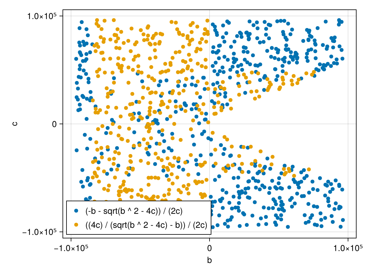
Infer good regimes
If we were to pick the best candidate expression for every point, we would end up with a lot of costly if-statements, and overfit on the points that we evaluated the expression with. To avoid excessive branching/overfitting we try to infer better regimes to split the domain.
julia> regimes = OptiFloat.infer_regimes(candidates, features["b"], points)OptiFloat.PiecewiseRegime{Vector{OptiFloat.Regime{Float16, OptiFloat.Candidate{DynamicExpressions.ExpressionModule.Expression{Float16, DynamicExpressions.NodeModule.Node{Float16}, @NamedTuple{operators::DynamicExpressions.OperatorEnumModule.OperatorEnum{Tuple{typeof(-), typeof(^), typeof(/), typeof(*), typeof(+)}, Tuple{typeof(-), typeof(sqrt), typeof(cbrt), typeof(log), typeof(exp), typeof(abs)}}, variable_names::Vector{String}}}, Vector{Float16}, OptiFloat.var"#toexpr#1"{DynamicExpressions.OperatorEnumModule.OperatorEnum{Tuple{typeof(-), typeof(^), typeof(/), typeof(*), typeof(+)}, Tuple{typeof(-), typeof(sqrt), typeof(cbrt), typeof(log), typeof(exp), typeof(abs)}}, Vector{String}}}, Vector{Bool}}}}(OptiFloat.Regime{Float16, OptiFloat.Candidate{DynamicExpressions.ExpressionModule.Expression{Float16, DynamicExpressions.NodeModule.Node{Float16}, @NamedTuple{operators::DynamicExpressions.OperatorEnumModule.OperatorEnum{Tuple{typeof(-), typeof(^), typeof(/), typeof(*), typeof(+)}, Tuple{typeof(-), typeof(sqrt), typeof(cbrt), typeof(log), typeof(exp), typeof(abs)}}, variable_names::Vector{String}}}, Vector{Float16}, OptiFloat.var"#toexpr#1"{DynamicExpressions.OperatorEnumModule.OperatorEnum{Tuple{typeof(-), typeof(^), typeof(/), typeof(*), typeof(+)}, Tuple{typeof(-), typeof(sqrt), typeof(cbrt), typeof(log), typeof(exp), typeof(abs)}}, Vector{String}}}, Vector{Bool}}[(E=0.02585, -Inf < b <= -0.1265) : ((4.0 * c) / (sqrt((b ^ 2.0) - (4.0 * c)) - b)) / (2.0 * c)
, (E=0.002012, -0.1265 < b <= Inf) : ((b * -1.0) - sqrt((b ^ 2.0) - (4.0 * c))) / (2.0 * c)
])julia> OptiFloat.print_report(stdout, original, regimes) ──────────────────────────────────────────────────────────────────────────────
OptiFloat Result
──────────────────────────────────────────────────────────────────────────────
Original Expression:
╭──────────────┬─────────┬──────────────────────────────────────╮
│ Interval │ Error │ Expression │
├──────────────┼─────────┼──────────────────────────────────────┤
│ b: (-∞, ∞) │ 1.305 │ (b * -1 - sqrt(b ^ 2 - 4c)) / (2c) │
╰──────────────┴─────────┴──────────────────────────────────────╯
Optimized PiecewiseRegime:
╭───────────────────┬────────────┬──────────────────────────────────────────╮
│ Intervals │ Error │ Expression │
├───────────────────┼────────────┼──────────────────────────────────────────┤
│ b: (-∞, -0.126) │ 0.02585 │ ((4c) / (sqrt(b ^ 2 - 4c) - b)) / (2c) │
├───────────────────┼────────────┼──────────────────────────────────────────┤
│ b: (-0.126, ∞) │ 0.002012 │ (b * -1 - sqrt(b ^ 2 - 4c)) / (2c) │
├───────────────────┼────────────┼──────────────────────────────────────────┤
│ Combined │ 0.014 │ % │
╰───────────────────┴────────────┴──────────────────────────────────────────╯
Improved function:
──────────────────────────────────────────────────────────────────────────────
function f(b, c)
begin
if -Inf16 < b <= Float16(-0.1265)
return ((4c) / (sqrt(b ^ 2 - 4c) - b)) / (2c)
end
if Float16(-0.1265) < b <= Inf16
return (b * -1 - sqrt(b ^ 2 - 4c)) / (2c)
end
end
end
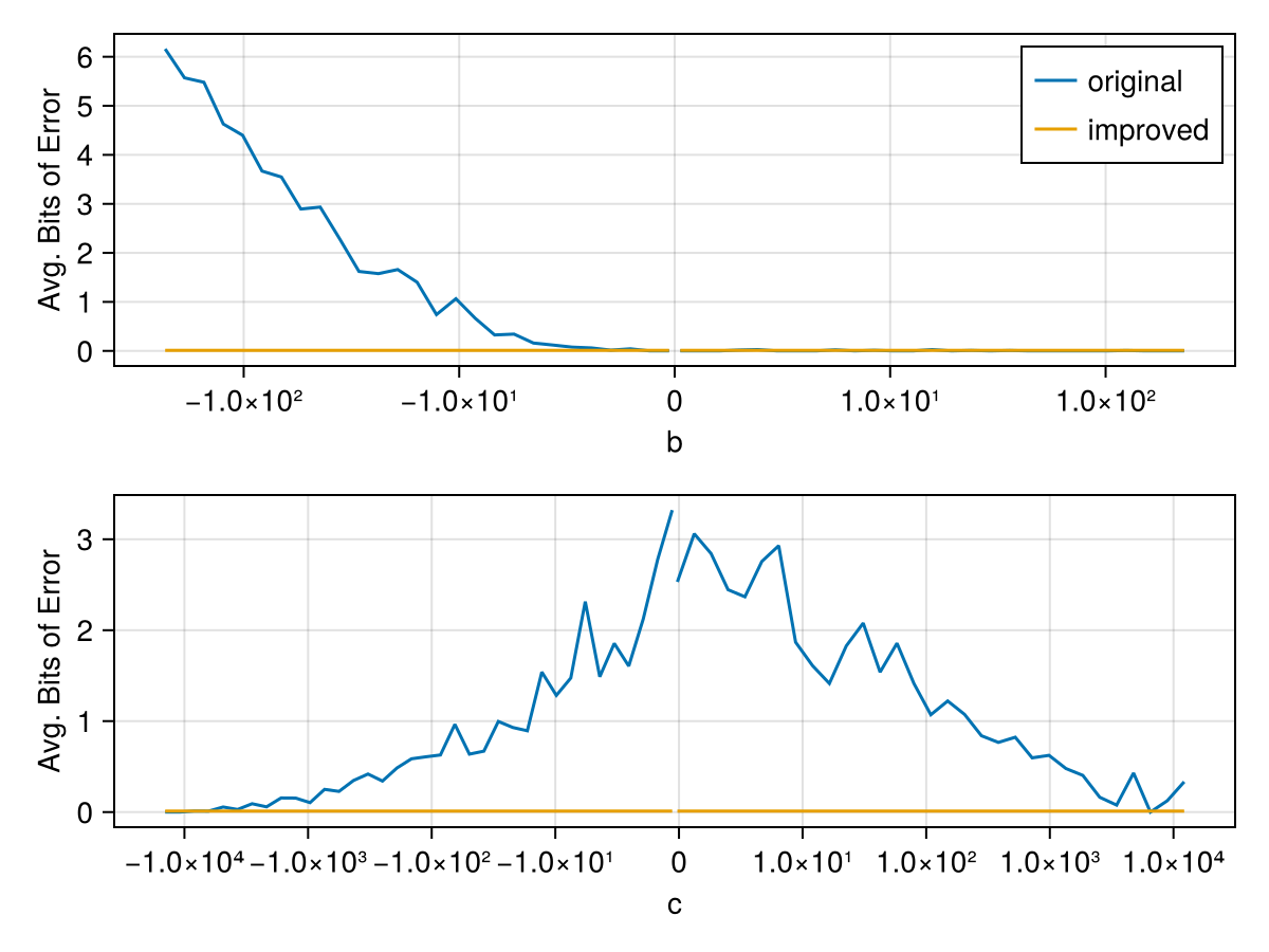
────────────────────────────────────────────────────────────────────────────── As we can see, OptiFloat splits the domain close to zero, which is exactly what we want.
Julia function of result expression
You immediately use the Julia function that is printed as part of the result:
julia> improved_expr = OptiFloat.regimes_to_expr(regimes)
:((b, c)->begin
          if -Inf16 < b <= Float16(-0.1265)
              return ((4c) / (sqrt(b ^ 2 - 4c) - b)) / (2c)
          end
          if Float16(-0.1265) < b <= Inf16
              return (b * -1 - sqrt(b ^ 2 - 4c)) / (2c)
          end
      end)

julia> improved_func = eval(improved_expr)
#1 (generic function with 1 method)

julia> improved_func(Float16(-1), Float16(-1))
Float16(0.618)
To verify that the resulting improved_func is actually performing better you can use the biterror function. The file scripts/arity-2.jl contains this workflow as a standalone script, including some plotting code to generate the error comparison below: